
| 일 | 월 | 화 | 수 | 목 | 금 | 토 |
|---|---|---|---|---|---|---|
| 1 | 2 | 3 | 4 | |||
| 5 | 6 | 7 | 8 | 9 | 10 | 11 |
| 12 | 13 | 14 | 15 | 16 | 17 | 18 |
| 19 | 20 | 21 | 22 | 23 | 24 | 25 |
| 26 | 27 | 28 | 29 | 30 | 31 |
- 프로그래머스
- 웹크롤링
- cnn
- 기계학습
- kaggle
- 에이블러
- 소셜네트워크분석
- 다변량분석
- 하계인턴
- 한국전자통신연구원 인턴
- Ai
- 빅분기
- httr
- ML
- 가나다영
- KT 에이블스쿨
- arima
- 딥러닝
- 서평
- Eda
- 에이블스쿨
- hadoop
- 지도학습
- python
- ggplot2
- 시각화
- 머신러닝
- dx
- KT AIVLE
- SQL
- 한국전자통신연구원
- 시계열
- 빅데이터분석기사
- kt aivle school
- 하둡
- matplot
- 에트리 인턴
- r
- ETRI
- SQLD
- Today
- Total
소품집
좌표계 변환하여 시공간 시각화 및 solar radiation 시각화 본문
KETR은 천리안 위성 기반 전국 전일사량 데이터를 제공하고 있는데, 천리안 1호 위성 데이터는 2012년 1월부터 2019년 12월까지, 천리안 2호 위성 데이터는 2019년 9월부터 2020년 8월까지 데이터를 제공하고 있음.
1. 데이터 다운로드
https://www.data.go.kr/data/15066413/fileData.do
2. 데이터 불러오기
import matplotlib.pyplot as plt
import seaborn as sns
import geopandas as pgd
import numpy as np
import pandas as pd

# 시각화 설정
sns.set_context('talk')
sns.set_style('white')

# 한글 사용 설정
plt.rcParams['font.family'] = ['NanumGothic', 'sans-serif']
plt.rcParams['axes.unicode_minus'] = False

df = pd.read_csv('C:\\Users\\user\\Desktop\\data\\한국에너지기술연구원_신재생자원지도데이터_태양자원_천리안1호_수평면전일사량_20191231.csv',
                 encoding = 'euc-kr') # 한글 인코딩
- 맑음 고딕 폰트가 없어서 시각화 시 아래와 같은 오류가 났다.
findfont: Font family ['NanumGothic'] not found. Falling back to DejaVu Sans.

import matplotlib
matplotlib.matplotlib_fname() # font 경로 확인: 'C:\\Users\\user\\anaconda3\\envs\\py_38\\lib\\site-packages\\matplotlib\\mpl-data\\matplotlibrc'
matplotlibrc 파일을 메모장으로 파일 열어서 #font.family를 설치해 준 폰트명으로 변경하면 된다.
그리고 ttf 폴더에 설치한 폰트도 옮겨주고 커널 재실행하면 됨.
df.to_pickle('C:\\Users\\user\\Desktop\\data\\KIER.pkl') # 백업
df.head()
df.shape # (291924, 98)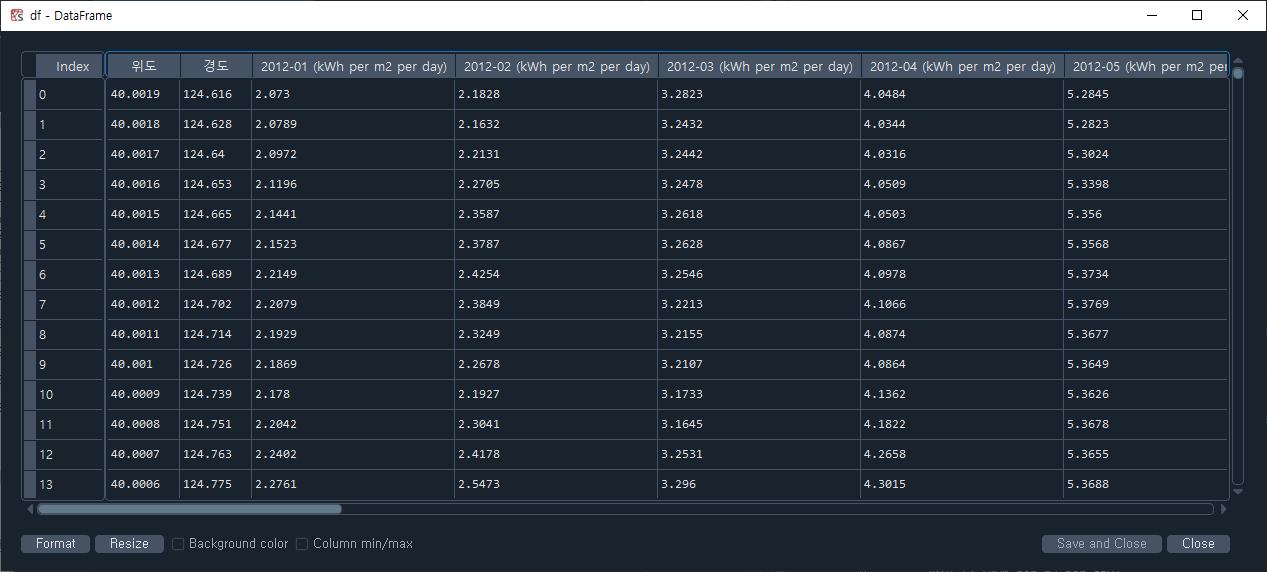
먼저 컬럼명에 단위를 삭제해 줬다.
공백을 기준으로 분리하여 첫 번째 문자열만 가져오도록 한다.
cols = list(df.columns)
cols_short = ['lon', 'lat'] + [c.split(' ')[0] for c in cols[2:]]
df.columns = cols_short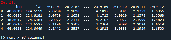
- 직진에 의해 태양으로부터 전달되는 일사량과 구름에 의해 산란된 일사량을 합친 값임.
- KETR에서는 도메인 지식 기반으로 계산하여 추론한다고 한다.
3. 시간에 대한 변환
3.1. 광주광역시 데이터 추출
- 광주광역시의 좌표는 북위 35.1595º, 동경 126.8526º
- 광주광역시와 가장 가까이 위치한 좌표를 찾으려면 위도와 경도 모두 가까워야 하므로 제곱의 합이 최소인 지점을 구해야 함.
# 광주 광역시 위경도 : 35.1595° N, 126.8526° E
idx = np.argmin(np.power(df['lonn']-35.1595, 2) + np.power(df['lat']-126.8526, 2))
df.iloc[idx]

# 시간에 대한 일사량을 확인하기 위해 시간과 일사량 데이터 가져오기
months = list(df.columns)[2:]
irrs = df.iloc[idx][2:]

fig, ax = plt.subplots(figsize = (10, 4))

# x축 범위 지정
ax.set_xlim(0, len(months)-1)

# x축 눈금 간격 지정
ax.xaxis.set_major_locator(MultipleLocator(12))

fig, ax = plt.subplots(figsize=(24, 8))
ax.plot(months, irrs, c='orange')
ax.set_title('수평면 전일사량 [kWh/(m$^2 \cdot$day)]', pad=10)
ax.set_xlim(0, len(months)-1)
ax.xaxis.set_major_locator(MultipleLocator(12))

# x축과 y축 눈금 글자 크기 축소
ax.tick_params(axis='both', labelsize='small')

# x축 눈금에서 grid 생성
ax.grid(axis='x')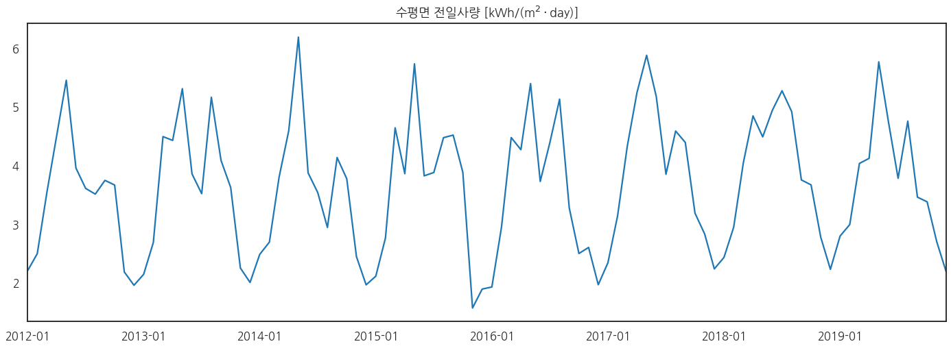
- ax.stackplot()으로 선 아래를 채색해 보자.
# stackplot
fig, ax = plt.subplots(figsize=(12, 4))

# stackplot
ax.stackplot(months, irrs, color='orange', ec = 'brown', alpha=0.5)

ax.set_title('수평면 전일사량 [kWh/(m$^2 \cdot$day)]', pad=10)
ax.set_xlim(0, len(months)-1)
ax.xaxis.set_major_locator(MultipleLocator(12))
ax.tick_params(axis='both', labelsize='small') # x, y축 글자 축소
ax.grid(axis='x') # x축에 grid 생성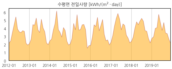
4. 공간 분포
4.1. scatter plot
- 한반도를 포함한 주변 영역의 데이터를 2차원에서 그려보자.
fig, ax = plt.subplots(figsize=(5, 6.67), constrained_layout=True)
ax.scatter(df['lat'], df['lon'], c=df['2012-01'], cmap='inferno')
ax.set_aspect('equal')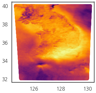
* 종횡비(aspect ration)를 1대 1로 맞췄음에도 불구하고 왜곡이 있음.
4.2. 좌표계 변환
- 위도와 경도는 곡면상에 놓였기 때문에 2차원으로 그리면 왜곡이 발생함.
- pyproj 라이브러리를 활용해 UTM-K 좌표계로 변경해 보자.
* UTM-K 좌표계는 대한민국에서 사용하는 좌표계 중 하나로, “Universal Transverse Mercator-Korean”의 약자로, 전 세계적으로 널리 사용되는 UTM 좌표계를 한반도에 맞게 변형한 것임.
from pyproj  import Transformer

transformer = Transformer.from_crs('epsg:4326', 'epsg:5178')
coord_UTMK = transformer.transform(df['lon'],df['lat'])
coord_UTMK

df_u = pd.DataFrame(data=np.array(coord_UTMK).T, columns=['y', 'x'])
df_u = pd.concat([df_u, df.iloc[:, 2:]], axis=1)
df_u.head() # 변경된 좌표계를 기존 데이터에 붙여 데이터 프레임을 만듦.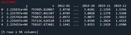
4.3. UTM-K 좌표계 기반 scatter plot
fig, ax = plt.subplots(figsize=(5, 6.67), constrained_layout=True)
ax.scatter(df_u['x'], df_u['y'], c=df_u['2012-01'], cmap='inferno')
ax.set_aspect('equal')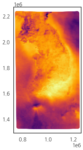
- 경기 동북부~강원도 서부 지역을 확대해 보자.
fig, ax = plt.subplots(figsize=(5, 6.67), constrained_layout=True)
ax.scatter(df_u['x'], df_u['y'], c = df_u['2012-01'], cmap='inferno')
ax.set_aspect('equal')
ax.set_xlim(1e6, 1e6+10000)
ax.set_ylim(2e6, 2e6+10000)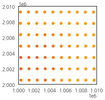
- 아래쪽이 붉어 보임. 좀 더 넓게 보자.
fig, ax = plt.subplots(figsize=(5, 6.7), constrained_layout=True)
ax.scatter(df_u['x'].iloc[:1000],
           df_u['y'].iloc[:1000],
           c = df_u['2012-01'].iloc[:1000], cmap='inferno')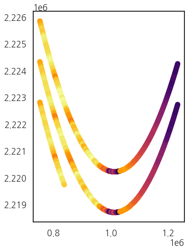
- (나는 이 시각화를 잘 해석하지 못하겠는데, 참고한 포스팅을 참조해 보자면 가로 세로가 맞지 않고, 좌표 변환의 이유라고 한다..)
4.4. 2D image 변환
- x, y (lon, lat) 2차원 데이터를 2D로 표현하는 가장 정석적인 방법은 meshgrid를 만드는 것.
- 위성 영상은 x, y 위치가 조금씩 틀어져있기 때문에 grid를 만들기 적절하지 않은데, 이때 사용하는 게 triplot, tricontourf, tricontour
- 샘플링해서 그려보자.
# 2D image 변환
df_us = df_u.sample(100)

# visualize
fig, axs = plt.subplots(ncols=3, figsize=(9, 6.67), sharex=True, sharey=True, constrained_layout=True)
axs[0].triplot(df_us['x'], df_us['y'], lw=0.5)
axs[1].triplot(df_us['x'], df_us['y'], lw=0.5, c='w')
axs[2].triplot(df_us['x'], df_us['y'], lw=0.5, c='k', alpha=0.5)

axs[1].tricontourf(df_us['x'], df_us['y'], df_us['2012-01'], cmap='inferno', levels=5)
axs[2].tricontour(df_us['x'], df_us['y'], df_us['2012-01'], cmap='inferno', levels=5)

for ax, title in zip(axs, ['triplot', 'tricontourf', 'tricontour']) :
    ax.set_aspect('equal')
    ax.set_title(title, pad=20)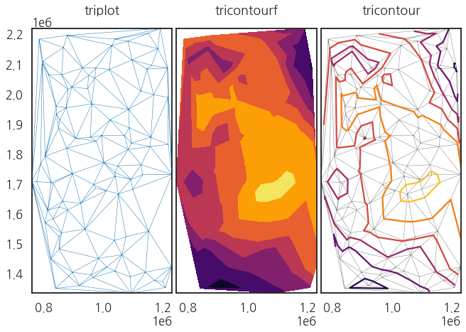
- ax.triplot() 은 주어진 (x, y) 데이터끼리 연결해 삼각형 mesh를 만듦.
- ax.tricontourf()는 (x, y) 위치데이터에서 node의 값 데이터를 적용해 삼각형 내 interpolation(보간법)을 함.
- levels을 5로 지정했기 때문에 다섯 개의 색상으로 표시되어 있고, 이게 경계선이 됨.
- ax.tricontour()는 이 경계선에 contour line을 그림.
fig, axs = plt.subplots(ncols=2, figsize=(6, 6.67), sharex=True, sharey=True, constrained_layout=True)

axs[0].tricontourf(df_u['x'], df_u['y'], df_u['2012-01'], cmap='inferno', levels=10)
axs[1].tricontourf(df_u['x'], df_u['y'], df_u['2012-01'], cmap='inferno', levels=10)

for ax, title in zip(axs, ['tricontourf', 'tricontoure']) :
    ax.set_aspect('equal')
    ax.set_title(title, pad=20)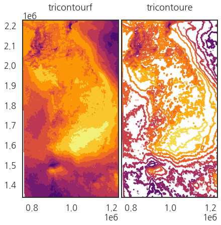
- levels을 10개로 설정하면 더 많은 구간을 확인해 볼 수 있음.
4.5. 지도 윤곽선 표시 (1) geopandas dataset
- geopandas 라이브러리에는 세계 지도와 주요 도시가 있음.
- 이를 활용해 한반도와 주변국의 윤곽선을 그려보자.
import geopandas as gpd

fig, ax = plt.subplots()
world[world['name']=='South Korea'].plot(ax=ax)
cities[cities['name']=='Seoul'].plot(ax=ax, c='yellow')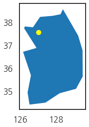
- x, y 축은 위경도이므로, UTM-K 좌표계로 데이터를 변환해 보자
# 좌표계 변환 by UTM-K
world = world.to_crs('EPSG:5178')
cities = cities.to_crs('EPSG:5178')

# 시각화
fig, ax = plt.subplots()
world[world['name']=='South Korea'].plot(ax=ax)
cities[cities['name']=='Seoul'].plot(ax=ax, c='yellow')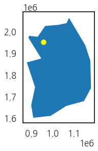
- 좌표계가 변환됐으면 일사량 데이터와 겹쳐보자.
fig, ax = plt.subplots(figsize=(5, 6.67), constrained_layout=True)
ax.tricontourf(df_u['x'], df_u['y'], df_u['2012-01'], cmap='inferno', levels=10)
ax.set_aspect('equal')

world[world['name']=='South Korea'].plot(ax=ax, fc='none', ec='w')
world[world['name']=='North Korea'].plot(ax=ax, fc='none', ec='w')
world[world['name']=='Japan'].plot(ax=ax, fc='none', ec='w')

ax.set_xlim(df_u['x'].min(), df_u['x'].max())
ax.set_ylim(df_u['y'].min(), df_u['y'].max())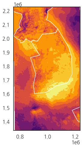
그래서 방법 2
4.6. 지도 윤곽선 표시 (2) shape file
- 행정구역 시도 경계선 데이터를 가져오자. 나는 가장 최신인 2023년 2월 업데이트 버전으로 다운로드했다.
- 대한민국 최신 행정구역(SHP) : http://www.gisdeveloper.co.kr/?p=2332
대한민국 최신 행정구역(SHP) 다운로드 – GIS Developer
www.gisdeveloper.co.kr
df_shp = gpd.read_file('C:\\Users\\user\\Desktop\\data\\CTPRVN_202302\\ctp_rvn.shp', encoding='euc-kr')
df_shp.head()
df_shp.columns

ax = df_shp.plot()
fig = ax.figure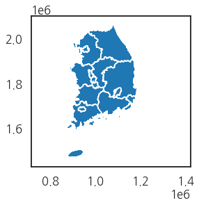
4.7. 일사량 데이터와 overlap
- 다시 2012년 1월 데이터에 겹쳐보자.
fig, ax = plt.subplots(figsize=(5, 6.67), constrained_layout=True)

ax.tricontourf(df_u['x'], df_u['y'], df_u['2012-01'], cmap='inferno', levels=10)
ax.set_aspect('equal')

df_shp.plot(ax=ax, fc='none', ec='w', lw=1, alpha=0.5)

ax.set_xlim(df_u['x'].min(), df_u['x'].max())
ax.set_ylim(df_u['y'].min(), df_u['y'].max())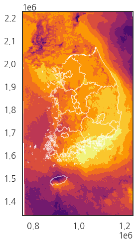
- 1월 데이터를 그려봤으니, 7월 데이터도 그려보자
fig, axs = plt.subplots(ncols=2, figsize=(10, 6.67), constrained_layout=True, sharex=True, sharey=True)

im0 = axs[0].tricontourf(df_u['x'], df_u['y'], df_u['2012-01'], cmap='inferno', levels=10)
im1 = axs[1].tricontourf(df_u['x'], df_u['y'], df_u['2012-07'], cmap='inferno', levels=10)

for ax, im, month in zip(axs, [im0, im1], ['2012-01', '2012-07']) :
    df_shp.plot(ax=ax, fc='none', ec='w', lw=1, alpha=0.5, zorder=2)
    im = ax.tricontourf(df_u['x'], df_u['y'], df_u[month], cmap='inferno', levels=10)
    ax.set_aspect('equal')
    ax.set_title(month, pad=20)
    ax.set_xlim(df_u['x'].min(), df_u['x'].max())
    ax.set_ylim(df_u['y'].min(), df_u['y'].max())

    plt.colorbar(im, ax=ax)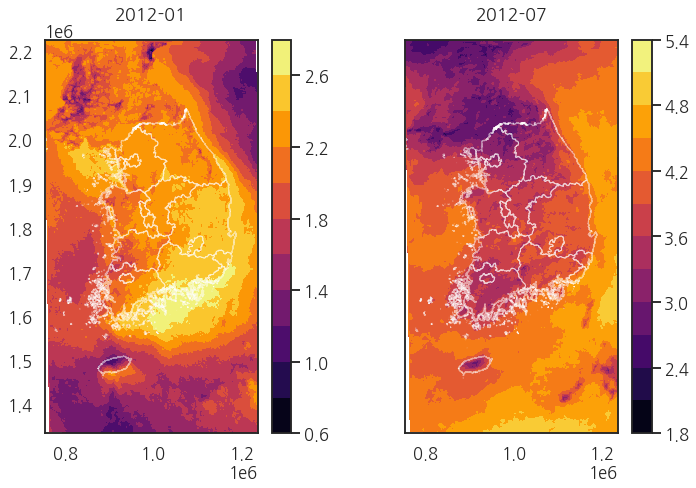
- 1월과 7월의 최소-최댓값이 다르므로 colormap의 최소 최댓값을 동일하게 지정해서 다시 그려보면,
# vmin=0, vmax=6
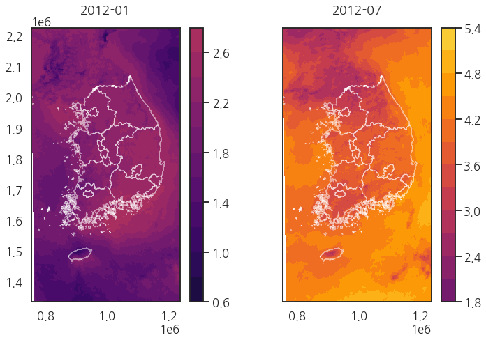
- 1월에 비해 7월에 더 많은 일사량을 띔.
5. 시간과 공간 데이터 시각화
- 공간 데이터는 1개월마다 평균치를 저장하므로 시간에 따른 변화를 확인해 볼 수 있음.
- 2012년부터 1월~12월까지의 공간 데이터를 확인해 보자.
from matplotlib import cm

fig, axes = plt.subplots(ncols=6, nrows=2, figsize=(10, 6), constrained_layout=True, sharex=True, sharey=True)

axs= axes.ravel()

for i, ax in enumerate(axs, 1) :
    month = f'2012-{i:02d}'
    df_shp.plot(ax=ax, fc='none', ec='w', lw=1, alpha=0.5, zorder=2)
    im = ax.tricontourf(df_u['x'], df_u['y'], df_u[month], cmap='inferno', levels=10, vmin=0, vmax=6)
    ax.set_aspect('equal')
    ax.set_title(month, pad=10)
    ax.set_xlim(df_u['x'].min(), df_u['x'].max())
    ax.set_ylim(df_u['y'].min(), df_u['y'].max())
    ax.axis(False)

# colarbar
# ScalarMappable()로 공통적인 colarbar 적용

cbar = cm.ScalarMappable(cmap='inferno')
cbar.set_clim(0, 6)
plt.colorbar(cbar, ax=axes[:, -1], fraction=0.2, pad=0.15)

# figure title
fig.suptitle('수평면 전일사량 [kWh/(m$^2 \cdot$day)]', color='gray', fontsize='medium', fontweight='bold')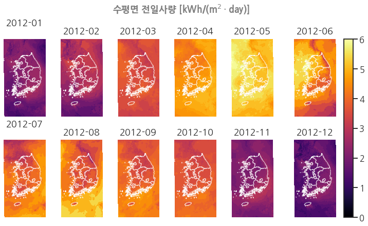
캐글 스터디방에서 좋은 정보를 많이 알려주시는 이제현 연구원님의 블로그에서 본 글인데,
태양 에너지, 일사량 등등 예측할 때 시각화 자료로 사용할 수 있을 것 같아서 필사해 봤다.
본 포스팅은 https://jehyunlee.github.io/2021/11/09/Python-DS-88_gpd_mpl/ 을 참조하며 좌표계 변환 및 시각화를 공부하며 실습해 봄
'AI' 카테고리의 다른 글
| 취준하는 자세와 마음 (1) | 2024.08.25 |
|---|---|
| GHI(Global Horizontal Irradiance), DNI(Direct Normal Irradiance), DHI(Diffuse Horizontal Irradiance) 정의 및 차이 (0) | 2023.04.22 |
| [tensorflow] TensorBoard 연동해서 학습률 확인하기 (0) | 2023.03.16 |
| [환경 설정] Tensorflow NVIDIA GPU 잡기, CUDA, cuDNN 설치 (0) | 2023.03.06 |
| [python] SHAP (SHapley Additive exPlanations), 설명 가능한 인공지능 (2) (0) | 2023.02.21 |


