
| 일 | 월 | 화 | 수 | 목 | 금 | 토 |
|---|---|---|---|---|---|---|
| 1 | 2 | 3 | 4 | |||
| 5 | 6 | 7 | 8 | 9 | 10 | 11 |
| 12 | 13 | 14 | 15 | 16 | 17 | 18 |
| 19 | 20 | 21 | 22 | 23 | 24 | 25 |
| 26 | 27 | 28 | 29 | 30 | 31 |
Tags
- KT AIVLE
- 머신러닝
- SQLD
- kt aivle school
- 빅분기
- 에이블스쿨
- ggplot2
- Eda
- ML
- 서평
- 프로그래머스
- 한국전자통신연구원 인턴
- SQL
- hadoop
- 다변량분석
- KT 에이블스쿨
- 에이블러
- 시각화
- 웹크롤링
- kaggle
- httr
- python
- dx
- 에트리 인턴
- 시계열
- 소셜네트워크분석
- Ai
- 기계학습
- matplot
- r
- 지도학습
- 하둡
- cnn
- 하계인턴
- 한국전자통신연구원
- 가나다영
- ETRI
- 빅데이터분석기사
- 딥러닝
- arima
Archives
- Today
- Total
소품집
[Kaggle] House prices 예측 (3) - 오늘은 실패 본문
728x90
오늘은 ..
수준보다 높은 kaggle notebook을 택한 탓인지 진행이 잘 안되어
다음번에 다시 도저어어언
+ ggolot2 option은 진짜 다양해서 그때마다 필요한 거 구글링 하는 게 최고옹
getwd()
setwd('/Users/dayeong/Desktop/reserch/data')
# Kaggle 3DAY
# https://www.kaggle.com/erikbruin/house-prices-lasso-xgboost-and-a-detailed-eda
# House prices : Laso, XGBoost, and a detailed EDA
# 주택 임대가격 예측하여 최종 가격 예측하기!
#
# Loading and Exploring Data
library(knitr)
library(ggplot2)
library(plyr)
library(dplyr)
library(corrplot)
library(caret)
library(gridExtra)
library(scales)
library(Rmisc)
library(randomForest)
library(psych)
library(xgboost)
library(ggrepel)
train <- read.csv('train.csv', stringsAsFactors = F)
test <- read.csv('test.csv', stringsAsFactors = F)
# Data size and structure
dim(train) ## 1460 by 81
str(train[,c(1:10, 81)]) # display first 10 variables and the response variable
# ID 제거 -> 예측시 필요치 않음
test_label <- train$Id
train$Id <- NULL
test$Id <- NULL
test$SalePrice <- NA # 우리가 예측하게 될 타겟 값인, 'SalePrice'
all <- rbind(train, test) # row_data set 생성
dim(all)
#
# Exploring some of the most important variable
# 마이닝 과정에서 필요한 중요 변수를 추출하기 위한 변수 selection
ggplot(data = all[!is.na(all$SalePrice),], aes(x=SalePrice)) +
geom_histogram(fill='blue', binwidth = 10000) +
scale_x_continuous(breaks = seq(0, 800000, by=100000), labels=comma)
summary(all$SalePrice)
# character variable을 살펴보기전, SalePrice와 상관관계를 갖는 숫자 변수를 알아보자.
# correlation(상관관계) with SalePrice
numericVars <- which(sapply(all, is.numeric)) # index vector numeric variable
numericVarNames <- names(numericVars)
cat('There are', length(numericVars), 'numeric variable')
all_numVar <- all[, numericVars]
cor_numVar <- cor(all_numVar, use='pairwise.complete.obs') # corr of numeric variable
# sort on decreasing correlation with saleprice - 상관관계 감소에 대해 분류해보자.
cor_sorted <- as.matrix(sort(cor_numVar[,"SalePrice"], decreasing = T)) # cor 내림차순 정렬
# select only high correlations
CorHigh <- names(which(apply(cor_sorted,1, function(x) abs(x) > 0.5)))
cor_numVar <- cor_numVar[CorHigh, CorHigh] # CorHigh 와 CorHigh의 상관계수 구하기.
corrplot.mixed(cor_numVar, tl.col='black', tl.pos = 'lt') # 변수간 상관성을 파악할 수 있게 됨.
# Overall Quality - (SalePrice와 가장 높은 상관계수를 보여주는 variable - 0.79)
# 시각화 결과 모든 각 등급별 집이 상승 추세를 보여주고 있음.
# 또한 특이값을 보이는 추정치는 없다 판단 가능.
ggplot(data=all[!is.na(all$SalePrice),], aes(x=factor(OverallQual), y=SalePrice)) +
geom_boxplot(col='blue') + labs(x='Overall Quality') +
scale_y_continuous(breaks= seq(0, 800000, by=100000), labels = comma)
# Above Grade (Ground) Living Area (square feet)
# Numeric variable 중 두 번째로 높은 cor보이는. 일반적으로 집이 넓으면 비싸다? -> 확인해보자.
# 특이치로, 524와 1299로 보인다.
ggplot(data=all[!is.na(all$SalePrice),], aes(x=GrLivArea, y= SalePrice)) +
geom_point(col='blue') +
geom_smooth(method = 'lm', se=F, col='black', aes(group=1)) +
geom_text_repel(aes(label=ifelse(all$GrLivArea[!is.na(all$SalePrice)] >4500, rownames(all),'')))
##
# Missing data, label encoding , and factorizing variables.
# 먼저, Missingvalue count.
NAcol <- which(colSums(is.na(all)) > 0)
sort(colSums(sapply(all[NAcol],is.na)), decreasing = T)
# Imputing missing data
# 1. Pool variables
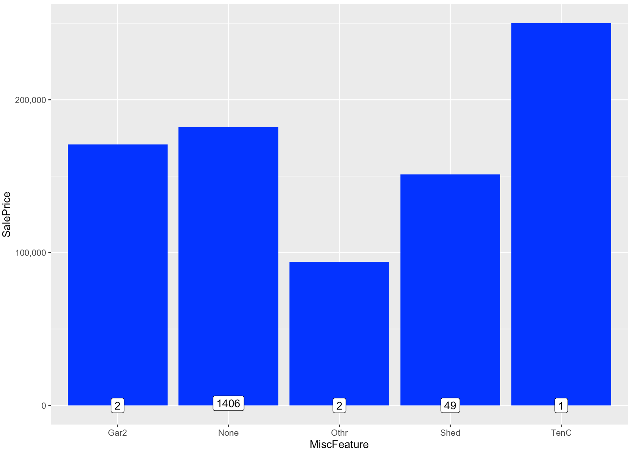
# 2. Miscekkaneous Feature
all$MiscFeature[is.na(all$MiscFeature)] <- 'None'
all$MiscFeature <- as.factor(all$MiscFeature)
ggplot(all[!is.na(all$SalePrice),], aes(x=MiscFeature, y=SalePrice)) +
geom_bar(stat='summary', fun.y = "median", fill='blue') +
scale_y_continuous(breaks= seq(0, 800000, by=100000), labels = comma) +
geom_label(stat = "count", aes(label = ..count.., y = ..count..))
table(all$MiscFeature) # summary count value ckeck.
# 3. Alley
all$Alley[is.na(all$Alley)] <-'None'
all$Alley <- as.factor(all$Alley)
ggplot(all[!is.na(all$SalePrice),], aes(x=Alley, y=SalePrice)) +
geom_bar(stat='summary', fun.y = "median", fill='blue')+
scale_y_continuous(breaks= seq(0, 200000, by=50000), labels = comma)
table(all$Alley)
# 4. Fence
all$Fence[is.na(all$Fence)] <- 'None'
table(all$Fence)
all[!is.na(all$SalePrice),] %>%
group_by(Fence) %>%
summarise(median = median(SalePrice), counts=n())
all$Fence <- as.factor(all$Fence)
# 5. Fireplace variable
all$FireplaceQu[is.na(all$FireplaceQu)] <- 'None'
all$FireplaceQu<-as.integer(revalue(all$FireplaceQu, Qualities))
table(all$FireplaceQu)
sum(table(all$Fireplaces))
# 6. Lot variables
all$LotFrontage[is.na(all$LotFrontage)] <- 'None'
ggplot(all[!is.na(all$LotFrontage),], aes(x=as.factor(Neighborhood), y=LotFrontage)) +
geom_bar(stat='summary', fun.y = "median", fill='blue') +
theme(axis.text.x = element_text(angle = 45, hjust = 1))
for (i in 1:nrow(all)){
if(is.na(all$LotFrontage[i])){
all$LotFrontage[i] <- as.integer(median(all$LotFrontage[all$Neighborhood==all$Neighborhood[i]], na.rm=TRUE))
}
}
all$LotShape<-as.integer(revalue(all$LotShape, c('IR3'=0, 'IR2'=1, 'IR1'=2, 'Reg'=3)))
table(all$LotShape)
sum(table(all$LotShape))
ggplot(all[!is.na(all$SalePrice),], aes(x=as.factor(LotConfig), y=SalePrice)) +
geom_bar(stat='summary', fun.y = "median", fill='blue')+
scale_y_continuous(breaks= seq(0, 800000, by=100000), labels = comma) +
geom_label(stat = "count", aes(label = ..count.., y = ..count..)) # 안 나오는데 ㅠㅠ
all$LotConfig <- as.factor(all$LotConfig)
table(all$LotConfig)
sum(table(all$LotConfig))
# 7. Garage vaiable
all$GarageYrBlt[is.na(all$GarageYrBlt)] <- all$YearBuilt[is.na(all$GarageYrBlt)]
length(which(is.na(all$GarageType) & is.na(all$GarageFinish) & is.na(all$GarageCond) & is.na(all$GarageQual))) # 157
# Find the 2 additional NAs
kable(all[!is.na(all$GarageType) & is.na(all$GarageFinish),
c('GarageCars', 'GarageArea', 'GarageType', 'GarageCond', 'GarageQual', 'GarageFinish')])
728x90
'AI' 카테고리의 다른 글
| [Kaggle] 채무 불이행자 searching - ing (4) (0) | 2020.08.31 |
|---|---|
| [Kaggle] interactive visualization (0) | 2020.08.28 |
| [Kaggle] Titanic 시각화 및 prediction (2) (0) | 2020.08.27 |
| [Kaggle] Airbnb Data시각화 및 regression (1) (0) | 2020.08.26 |
| [ML/DL] Topic modeling, LDA (0) | 2020.06.24 |
'AI' Related Articles
more


Comments